Mechanics: Fluids

Fluids: Problem Set Overview

There are eight ready-to-use problem sets on the topic of Fluids. Most problems are multi-part problems requiring an extensive analysis. The set of problems on this topic targets your ability to use the concepts of Newton’s Laws, the W=∆E relationships and the Conservation of Mass along with the definition of density and pressure to solve problems involving Hydrostatic Pressure and Hydrodynamics. Problems range in difficulty from the very easy and straight-forward to the very difficult and complex.

 

Some Definitions

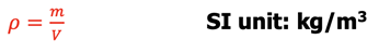
Density of a substance: The ratio of mass over volume and denoted by the Greek letter rho.

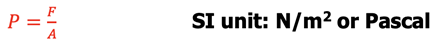
Pressure: How a contact force perpendicular to a surface is distributed over any small area.

 

 

Pressure in a Fluid

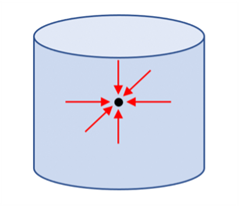It is an experimental observation that a fluid exerts pressure in any direction. At a given depth the pressure is the same in every direction in a nonmoving fluid. Consider a tiny ball of fluid in the middle of a cylindrical column of fluid as shown at right. The pressure on each side must equal the pressure on the opposite side. If this weren’t true, the fluid would be in motion.

Although pressure is a scalar the force due to fluid pressure always acts perpendicular to any solid surface it touches. If this weren’t true, the force component on the object from the fluid parallel to the surface would be part of a Newton’s 3^rd Law Action-Reaction pair of forces. There would then be a reaction force from the object back on the fluid, causing the fluid to move parallel to the surface. This is not observed.
 

Hydrostatic Pressure

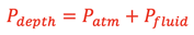
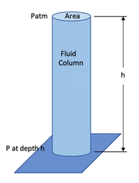Consider a cylindrical column of fluid sitting on a flat plate as shown at right. The fluid will exert a pressure, P_depth, on the face of that plate at a depth, h. To determine the absolute pressure on the plate the atmospheric pressure above the fluid column must be considered. The external atmospheric pressure exerted on the top of the fluid column is transmitted to the plate. This is a general principle attributed to Blaise Pascal. Pascal’s Principle states that if an external pressure is applied to a confined fluid, the pressure at every point within the fluid increases by that amount. The P at depth h can be calculated as follows.

and substitution for P_fluid gives

.

Since

,

then

.

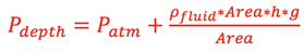Canceling the Area produces the following for the Hydrostatic Pressure at a depth h:

.

 

 

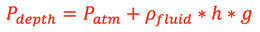Hydrostatic Force

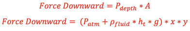
The pressure from the fluid column and atmosphere will combine to create a force downward on the plate involving P_depth multiplied by the cross-sectional area, A.

 

Buoyant Force on a Submerged Object

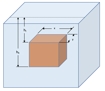Consider a block held in a fluid such that there is fluid above and below as shown at right. There will be opposing hydrostatic forces above and below the block with different pressures according to the distance of the top and bottom faces of the block below the fluid surface. The force pushing down on the top face from the fluid will be

,

and the force pushing up on the bottom face from the fluid will be

.

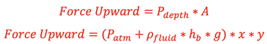All vertical faces of the block also experience a force from the fluid pressure. However, since the distance below the surface is equal for those faces the forces on opposite sides of the block will be equal and in opposite directions. Therefore, all horizontal vector forces due to fluid pressure would sum to 0. The lower surface experiences a greater pressure than the upper surface due to being deeper in the fluid. Therefore, the net force will be upwards on the block. This net force from the fluid is called the Buoyant Force. Its final value would be determined as follows:
 
This result is attributed to Archimedes. Archimedes’ Principle states that the buoyant force on an object immersed in a fluid is equal to the weight of the fluid displaced by that object.



 

Moving Fluid and the Conservation of Mass

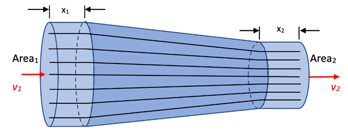
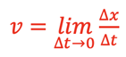
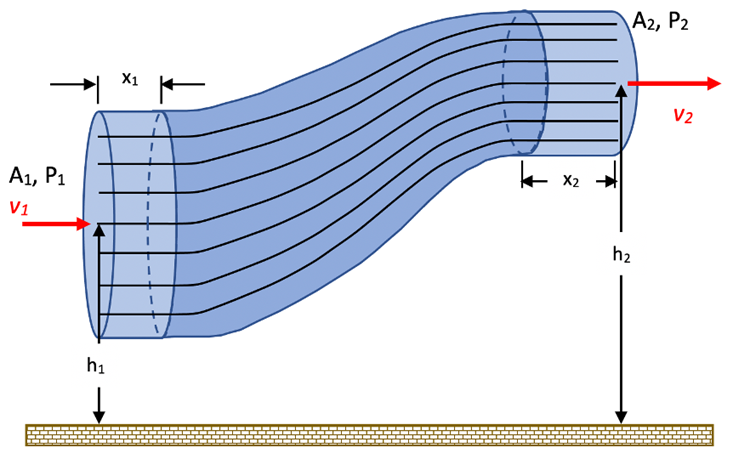
Let’s consider a fluid moving left to right through a differing diameter pipe in the horizontal direction as shown below. The lines drawn inside the pipe are called streamlines. A streamline represents fluid flow such that each particle of the fluid follows a smooth path, called a streamline, and these paths do not cross one another. The streamlines represent the flow of fluid particles moving into the left end with cross-sectional area, A₁, and eventually moving out the right end with cross-sectional area, A₂. Another phrase for this type of motion is Laminar Flow. Above a certain speed fluid will not follow these streamlines and become turbulent. This is referred to as Turbulent Flow and results in energy losses due to internal friction, also called viscosity. The following analysis is for incompressible fluid with negligible viscosity undergoing steady (constant density, velocity, and pressure at each point), laminar flow.
 

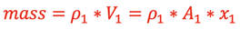
Consider the mass of fluid inside the pipe through the length, x₁, at an instant in time;

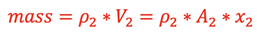
The length, x₂, is chosen such that this same amount of fluid will fully occupy the volume inside the pipe on the other end through the length, x₂. The mass at that instant in time will be

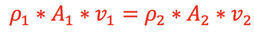
Therefore, since the mass is the same at these 2 different sections of the pipe,

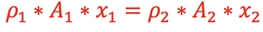
If we are dealing with incompressible fluids such as water, the density,ρ, will be the same throughout the pipe. Then,

.

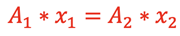In general, if an equal mass of fluid flows through very narrow sections of pipe, ∆x, in a small interval of time, ∆t, the relationship can be written as

,

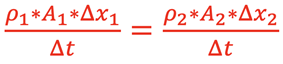and since

,

this can then be written as

.

This is referred to as the Continuity Equation. If we are dealing with incompressible fluids such as water, the density, ρ, will be the same throughout the pipe. Therefore, an equal mass of fluid existing at any 2 sections in the pipe will give

.

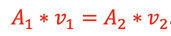This is the Continuity Equation for constant density fluids and is also called the Volume Flow Rate.




 

 

Moving Fluid and the Conservation of Energy

Let’s consider a fluid moving through a differing diameter pipe at different vertical positions as shown below. The streamlines represent the flow of fluid particles moving into the left end at speed, v₁, with cross-sectional area, A₁, and fluid pressure, P₁. These fluid particles eventually move out the right end at speed, v₂, with cross-sectional area, A₂, and fluid pressure, P₂.

Let’s start the analysis of the fluid flow using the Work=∆E relationship from previous experience.
 

The initial and final energy considerations include both potential and kinetic terms. Non-conservative Work is done by the initial pressure, P₁, being greater than the final pressure, P₂, or else the fluid would not flow as shown. Therefore, the next iteration of the equation looks like this: The following equations would pertain to an equal mass of fluid moving through this pipe assuming that the fluid completely takes up all of the volume in sections with lengths x₁ and x₂:
A previous result for the Conservation of Mass showed that A₁*x₁ = A₂*x₂. Using that result means that the A*x can be canceled in each term. That will produce the following Energy/Volume results:
Replacing all terms in the original equation with these results would give
 
The pressure at position 2 is putting force in the opposite direction of the fluid flow so the angle between the force and direction of motion is 180˚. This equation is called Bernoulli’s Equation and is usually written such that Position 1 is compared to Position 2 like this:
 


 

 

Fluids Mechanics’ Equations

We can now summarize our results from Hydrostatics and Hydrodynamics to produce the following for an incompressible fluid with steady, laminar flow:

 

 

 

Summary of Conditions for Fluids

One difficulty a student may encounter with this topic is the confusion as to which formula to use. When approaching these problems it is suggested that you practice the usual habits of an effective problem-solver; identify known and unknown quantities in the form of the symbols of physics formulas, plot out a strategy for using the knowns to solve for the unknown, and then finally perform the necessary algebraic steps and substitutions required for the solution.


 

Habits of an Effective Problem-Solver

An effective problem solver by habit approaches a physics problem in a manner that reflects a collection of disciplined habits. While not every effective problem solver employs the same approach, they all have habits which they share in common. These habits are described briefly here. An effective problem-solver...

• ...reads the problem carefully and develops a mental picture of the physical situation. If needed, they sketch a simple diagram of the physical situation to help visualize it.
• ...identifies the known and unknown quantities in an organized manner, often times recording them on the diagram itself. They equate given values to the symbols used to represent the corresponding quantity (e.g., ρ = 1.15 g/cm³, A = 2.5 L, m = ???).
• ...plots a strategy for solving for the unknown quantity. The strategy will typically centers around the use of physics equations and is heavily dependent upon an understanding of physics principles.
• ...identifies the appropriate formula(s) to use, often times writing them down. Where needed, they perform the needed conversion of quantities into the proper unit.
• ...performs substitutions and algebraic manipulations in order to solve for the unknown quantity.

Read more...