Mechanics: Rotational Kinematics
Rotational Kinematics: Problem Set Overview
We have 8 ready-to-use problem sets on the topic of Rotational Kinematics. These problem sets focus on the analysis of situations involving a rigid object rotating in either a clockwise or counterclockwise direction about a given point. The object's rotation speed may be increasing, decreasing, or remaining constant.
Characteristics of Objects in Rotational Motion
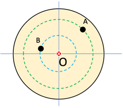 Objects in purely rotational motion involve rigid (non-deformable) objects that have a singular point around which all other points on the object complete a circular path in one complete rotation of the object. Consider Point O to be the axis of rotation in the object at right. Points A and B will follow the dotted circular paths if the object is rotated.
Angular Position and Angular Displacement
Consider the initial position of a point at position A on the x-axis as shown below left. After a period of time the point has rotated counterclockwise to its new position B shown below right. The point is now at an angular position of θ with reference to the x-axis. That angular position can be described in units of degrees or radians.
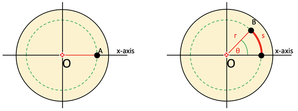
The radian is an angular measure that is defined by the ratio of the arc length traveled, s, divided by the radius, r, Expressed as an equation, it can be said θ = s/r.
There are 360˚ or 2π radians in a full circle. Therefore,

If a point is rotated around a fixed center on a rigid body from an initial position, A, to a final position, B, we say it has had an angular displacement. That would be evaluated as:

The quantity ∆θ would have a positive value if displaced counterclockwise and a negative direction if displaced clockwise.
Average and Instantaneous Angular Velocity
If a point is rotated around a fixed center on a rigid body from an initial angular position to a final angular position over a period of time, we say it has an average angular velocity, ωavg. That value would be evaluated as ωavg = ∆θ/∆t. A positive or negative calculation result would depend on the sign of ∆θ. The average angular speed would be the magnitude of the average angular velocity.
The instantaneous angular velocity of a rotating rigid object is mathematically defined as the limit of the average speed as the time interval ∆t approaches zero:

The instantaneous angular speed is the magnitude of the instantaneous angular velocity. When the angular speed is constant, the instantaneous angular speed is equal to the average angular speed.
Average and Instantaneous Angular Acceleration
If a point is rotated around a fixed center on a rigid body with an initial angular velocity, ωi, to a final angular velocity, ωi, over a period of time, we say it has an average angular acceleration, αavg. That value would be evaluated as αavg = ∆ω/∆t. A positive or negative calculation result would depend on the sign of ∆ω.
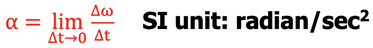
The instantaneous angular acceleration of a rotating rigid object is mathematically defined as the limit of the average acceleration as the time interval ∆t approaches zero:
When the angular acceleration is constant, the instantaneous angular acceleration is equal to the average angular acceleration.
Rotational Motion under Constant Angular Acceleration
The definitions for the rotational quantities, θ, ∆θ, ω, ∆ω, and α are similar to the definitions for the linear quantities, x, ∆x, v, ∆v, and a. Due to the rotational variables sharing the same mathematical relationships between them as the linear variables, new equations can be written for rotational motion that mimic the equations for linear motion.
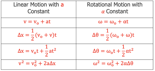
Every term in a specific linear equation has a corresponding term in the analogous rotational equation.
Relations between Angular and Linear Quantities
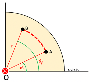
Consider a point P on an arbitrarily shaped, rigid object able to rotate counterclockwise around an axis of rotation at O in the z-direction. The point P starts on the x-axis at a radial distance of r and ends at the position shown below. That point will have rotated through an angular displacement, ∆θ, and an arc length, ∆s.
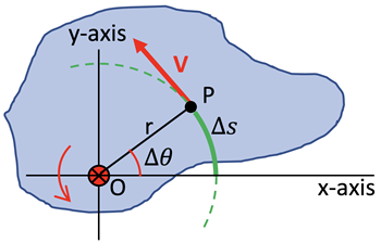
The relationship between r, ∆θ, and ∆s is the following:

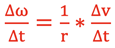
If the time interval to complete the rotation is ∆t, dividing both sides by this increment of time gives:
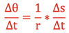
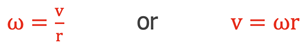
As the time interval, ∆t, approaches zero, the ratio on the left approaches the instantaneous angular velocity, ω, and the ratio on the right approaches the linear velocity, v, that becomes tangent to the curve. Performing these substitutions gives:
If point P started from rest, it experienced a change in angular and linear speed as it rotated from its original position. We can analyze this situation by dividing the previous equation by the time interval, ∆t.
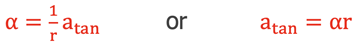
Once again as the time interval, ∆t, approaches zero, the ratio on the left approaches the instantaneous angular acceleration, α, and the ratio on the right approaches the linear acceleration, a, that becomes tangent to the curve. Performing these substitutions gives:
Summary of Conditions for Kinematic Rotational Motion
One difficulty a student may encounter with this topic is the confusion as to which formula to use. When approaching these problems it is suggested that you practice the usual habits of an effective problem-solver; identify known and unknown quantities in the form of the symbols of physics formulas, plot out a strategy for using the knowns to solve for the unknown, and then finally perform the necessary algebraic steps and substitutions required for the solution.
Linear and Rotational Relationships:
∆s = ∆θ•r
vtan = ω•r
atan = α•r
Rotational Big 4:
ω = ωo + α•t
∆θ = ½•(ωo + ω)•t
∆θ = ωo•t + ½•α•t2
ω2 = ωo2 + 2•α•∆θ
Habits of an Effective Problem-Solver
An effective problem solver by habit approaches a physics problem in a manner that reflects a collection of disciplined habits. While not every effective problem solver employs the same approach, they all have habits which they share in common. These habits are described briefly here. An effective problem-solver...
- ...reads the problem carefully and develops a mental picture of the physical situation. If needed, they sketch a simple diagram of the physical situation to help visualize it.
- ...identifies the known and unknown quantities in an organized manner, often times recording them on the diagram itself. They equate given values to the symbols used to represent the corresponding quantity (e.g., ∆θ = 0.982 rad, ωo = 0.0 rad/s, r = 0.251 m, ω = ???).
- ...plots a strategy for solving for the unknown quantity. The strategy will typically center saround the use of physics equations and is heavily dependent upon an understanding of physics principles.
- ...identifies the appropriate formula(s) to use, often times writing them down. Where needed, they perform the needed conversion of quantities into the proper unit.
- ...performs substitutions and algebraic manipulations in order to solve for the unknown quantity.
Read more...