Electricity: Transient RC Circuits
Transient RC Circuits: Problem Set Overview
We have four ready-to-use problem sets on the topic of Transient RC Circuits. Most problems are multi-part problems requiring an extensive analysis. The problems target your ability to apply concepts of potential, capacitance, resistance, and current in order to analyze transient RC circuits.
Electric Circuits
Circuit elements (Voltage sources, resistors, and capacitors) can be arranged into various configurations using conductive wires. The voltage across an element and the current in the element depend on the following principles and conventions.
- Positive charge will flow from high potential to low potential in a conductive circuit.
- Resistors can be assembled in series, parallel, and combination configurations.
- Resistor values are determined by physical characteristics: material, length, area.
- Capacitors can be assembled in series, parallel, and combination configurations.
- Capacitor values are determined by physical characteristics: dielectric, distance between plates, plate area.
- Once fully charged, capacitors act like an open in the circuit (no charge flow).
- When completely uncharged, capacitors act like a short in the circuit (unimpeded charge flow).
- Ohm’s Law and Kirchhoff’s Laws can be used to analyze circuit behavior.
Electric Circuit Schematic
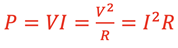
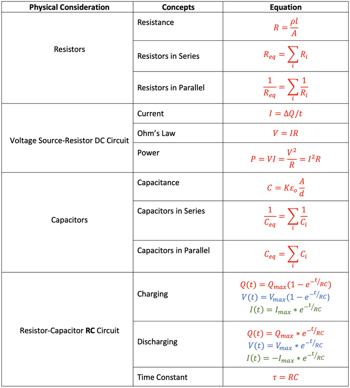
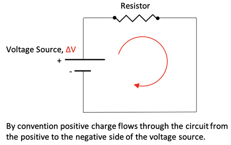 A simple circuit is shown at right. An individual resistor value can be calculated knowing the resistivity, length, and area of the resistor, R = ρ•L/A. Current is the rate of charge flow, I = ∆Q/t. The voltage drop across the resistor will equal the Source Voltage and the current in the resistor can be calculated using Ohm’s Law, V = I•R. Power dissipated in the resistor can be calculated using any of the following expressions:
Resistor Combinations
 Two resistors in series give the following results.
- Equivalent resistance: Req = R1 + R2
- Current: Itotal = I1 = I2
- Voltage Drop: Vtotal = V1 + V2
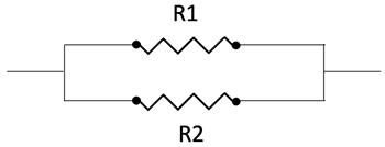
Two resistors in parallel give the following results.
- Equivalent resistance: Req = (R1-1 + R2-1)-1
- Current: Itotal = I1 + I2
- Voltage Drop: Vtotal = V1 = V2
Capacitor Charging
A capacitor can be wired in series with a resistor and voltage source to produce a resistor-capacitor (RC) circuit as shown below left. After closing the switch charge flow begins and produces a buildup of charge on the capacitor plates. The capacitor eventually causes the current to stop flowing in the circuit. This is because the charge buildup on the plates produces a voltage across the plates that is equal and opposing to the Voltage Source that originally moved the charge.

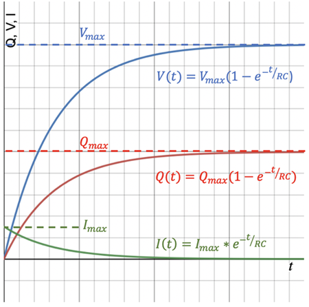 Kirchhoff’s Law and calculus can derive the charging equations for the RC circuit shown above. Those equations are shown with the associated curve at right. Qmax is the charge built up on the plates when the charging process is finished, Vmax is the final voltage across the plates that develops due to the charge buildup, and Imax is the initial rate of charge flow. The time-based equations are:
- Amount of charge on the plates: Q(t) = Qmax(1 – e-t/RC)
- Amount of voltage on the plates: V(t) = Vmax(1 – e-t/RC)
- Rate of charge flow in the circuit: I(t) = Imax • e-t/RC
The relationship between the maximum values is the following:
Qmax = C•Vmax, Vmax = Vsource, and Vsource = Imax•R
Capacitor Discharging
A charged capacitor can be wired in series with a resistor to produce the RC circuit as shown below left. After closing the switch, charge flow begins due to the Coulomb Force, thereby releasing the buildup of charge on the capacitor plates. The reduction in charge on the plates causes the voltage across the plates to decrease. This results in the charge on the plates and the voltage drop across the plates to diminish to zero.
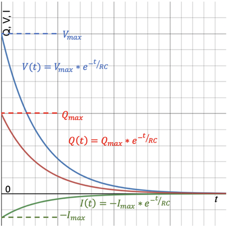
Kirchhoff’s Law and calculus can derive the discharging equations for the
RC circuit shown above. Those equations are shown with the associated curve at right.
Qmax is the initial charge built up on the plates before the discharging process begins,
Vmax is the initial voltage drop across the plates that developed due to the charge buildup, and
-Imax is the initial rate of charge flow. The negative sign indicates that the charge flow is in the opposite direction to the charge flow when charging the capacitor. The time-based equations are:
- Amount of charge on the plates: Q(t) = Qmax • e-t/RC
- Amount of voltage on the plates: V(t) = Vmax • e-t/RC
- Rate of charge flow in the circuit: I(t) = -Imax • e-t/RC
The relationship between the maximum values is the following:
Qmax = C•Vmax and Vmax = Imax•R
The Time Constant for RC Circuits
The multiplication of Resistance in Ohms multiplied by C in Farads results in a Time in Seconds. This product is referred to as the time constant, τ, for the circuit whether it is charging or discharging:
τ = R•C.
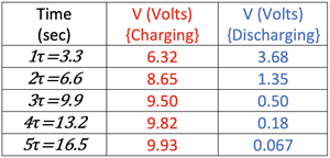
For practical purposes a circuit is considered charged or discharged after a period of five time constants. Let’s look at an analysis of the voltage across the plates in a discharging capacitor at multiples of the time constant.
The time-based voltage equation for a discharging capacitor is: V(t) = Vmax • e-t/RC
Let’s substitute
τ into the equation:
V(t) = Vmax • e-t/τ
The voltage at
t=τ: V(t) = Vmax • e-t/τ = Vmax • e-1 = 0.368•Vmax
The voltage at
t=2τ: V(t) = Vmax • e-t/τ = Vmax • e-2 = 0.135•Vmax
The voltage at
t=3τ: V(t) = Vmax • e-t/τ = Vmax • e-3 = 0.05•Vmax
The voltage at
t=4τ: V(t) = Vmax • e-t/τ = Vmax • e-4 = 0.018•Vmax
The voltage at
t=5τ: V(t) = Vmax • e-t/τ = Vmax • e-5 = 0.0067•Vmax
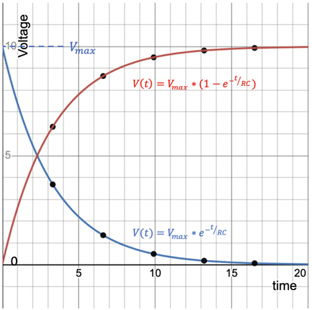
The time-based voltage curves for the charging and discharging situations are shown at right. The values for the voltage across the plates at the multiples of the time constant are plotted on the curves for the following values:
R = 1000 Ω
C = 3300 µf
τ = R•C = 3.3 s
Vmax = 10 Volts
Capacitor Combinations
Multiple capacitors can be arranged in circuits just like resistors; series, parallel, and a combination of the two.
Capacitors in Series: Let’s look at the charging of 2 identical capacitors in series compared to just 1 of them as shown in the circuits below.
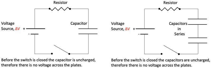
The circuits are shown below after the switch is closed and the capacitors are fully charged. Colored lines are used to represent the Electric Potential (Voltage) of the Voltage Source and the capacitors.
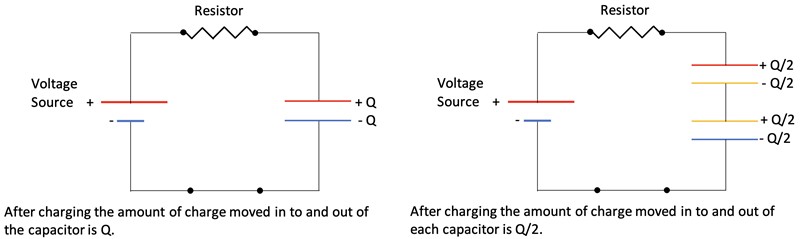
The voltage across the single capacitor is equal to the voltage source after charging. Due to Kirchhoff’s Voltage Law the voltage across an individual capacitor in the 2- capacitor circuit is half the voltage source. What does this say about the circuit overall capacitance? We can write the following equation after charge has stopped moving:
Vacross both caps = V1 + V2,
and since Q = C•V,
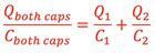
and since
Vboth caps = V1 = V2, the single capacitor that can replace two capacitors in series can be calculated by
Capacitors in Parallel: Let’s look at the charging of 2 identical capacitors in parallel compared to just 1 of them as shown in the circuits below.
The circuits are shown below after the switch is closed and the capacitors are fully charged. Colored lines are used to represent the Electric Potential (Voltage) of the Voltage Source and the capacitors.
The voltage across the single capacitor is equal to the voltage source after charging. The voltage across an individual capacitor in the 2- capacitor circuit is also the same as the voltage source. What does this say about the circuit overall capacitance? We can write the following equation after charge has stopped moving:
Qinto both caps = Q1 + Q2,
and since Q = C•V,
Cequivalent•Vsource = C1•V1 + C2•V2
and since Vsource = V1 + V2, the single capacitor that can replace two capacitors in parallel can be calculated by
Cequivalent = C1 + C2
Equation Summary
Habits of an Effective Problem-Solver
An effective problem solver by habit approaches a physics problem in a manner that reflects a collection of disciplined habits. While not every effective problem solver employs the same approach, they all have habits which they share in common. These habits are described briefly here. Effective problem-solvers ...
- ...read the problem carefully and develops a mental picture of the physical situation. If needed, they sketch a simple diagram of the physical situation to help visualize it.
- ...identify the known and unknown quantities in an organized manner, often times recording them on the diagram itself. They equate given values to the symbols used to represent the corresponding quantity (e.g., F = 0.025 N, E = 4.50x10⁻⁶ N/C, q = ???).
- ...plot a strategy for solving for the unknown quantity. The strategy will typically center around the use of physics equations and is heavily dependent upon an understanding of physics principles.
- ...identify the appropriate formula(s) to use, often times writing them down. Where needed, they perform the needed conversion of quantities into the proper unit.
- ...perform substitutions and algebraic manipulations in order to solve for the unknown quantity.
Read more...