Lesson 1: Physics in the Early 20th Century

Part c: Bohr's Quantized Energy Levels

Part 1a: Emission Spectrum of the Elements
Part 1b: The Photon
Part 1c: Bohr's Quantized Energy Levels
Part 1d: Wave-Particle Duality
 

 

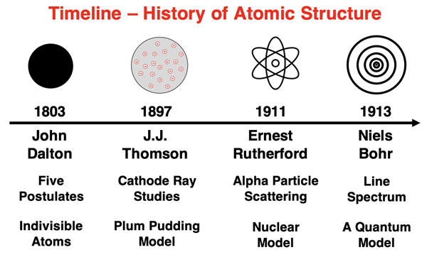
Early Atomic Models

Earlier models of the atom were discussed in Chapter 3 of this Chemistry Tutorial. John Dalton’s model from 1803 included 5 postulates about atoms but no discussion of its internal structure. JJ Thomson proposed the plum pudding model of the atom in 1897, suggesting the atom consisted of negatively charged particles embedded in a sea of positive charge. Ernest Rutherford proposed the first nuclear model in 1911, describing the atom as having negatively charged electrons orbiting about a densely packed nucleus of positive charge. And in 1913 Niels Bohr proposed that the orbiting electrons could orbit with only certain radii that were associated with quantized energy levels.
 
Bohr’s model was the first quantum model. It was an attempt to address the issues associated with the electron orbits of the Rutherford model. It was also an attempt to explain the emission spectra of the elements.
 

 
 
 

Mathematics of the Bohr Model

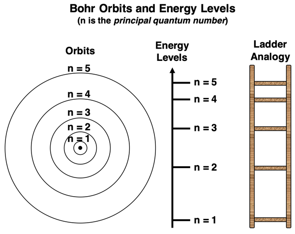
Niels Bohr’s quantum model assumed that the electron could only orbit with certain allowed radii. Each orbit was associated with an energy level. Because only certain orbits were allowed, the electron occupying those orbits could only have certain quantized energy levels. Bohr assigned a number to each orbit, known as the principal quantum number (n). Values of n were restricted to integer values (1, 2, 3, 4, etc.). A value of n = 1 was assigned to the lowest orbit, referred to as the ground state. A value of n = 2 was assigned to the orbit with the second largest radius. And so forth.
 
Bohr used equations from classical physics, like Newton’s second law equation and the Coulomb’s law equation of electrical interaction, to derive an equation relating the energy (E) of each orbit to the principal quantum number (n) of that orbit. The equation is:

 
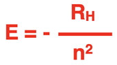
where R_H is the so-called Rydberg constant. The Rydberg constant applies only to the element hydrogen and has a value of 2.180 x 10^-18 J. In the derivation of his equation, Bohr assumes that the zero-energy location is that of an electron an infinite distance from the nucleus. All energy levels for electrons are values less than these zero energies. In other words, the energy values are negative.
 
The Bohr equation can be used to calculate the energy of an electron in any of the orbits. Two sample calculations are shown below for the n = 1 and n = 2 energy levels. The table shows the results for the first 10 energy levels of the hydrogen atom.

 
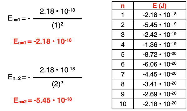
As can be seen in the data table above, the electron energies allowed by the Bohr atom are not equally spaced. If you think of quantum energy levels being analogous to rungs on a ladder, then the rungs are not equal distant apart. The rungs on the ladder get closer together as the n value increases to higher and higher levels. This is depicted in the graphic below. This means that progressing from one energy level up or down to the next energy level does not result in the same energy change.

 

 

 

Electron Transitions

The emission spectra of elements was discussed earlier in Lesson 1. When heat or electricity is applied to an element, its electrons absorb the energy and transition to higher energy states. These electrons eventually release the energy in quantized amounts as they relax back to a ground state.
 
Niels Bohr is attempting to provide an explanation for the emission spectrum of hydrogen. Each line corresponds to the release of a photon. The photon is released as the electron transitions from an excited state to a lower energy state. The energy change of the electron is equal to the energy of the photon that it releases. As Planck and Einstein suggested, the energy of such a photon is related to the frequency (f) and the wavelength (λ).

 
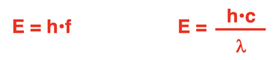
(h is Planck’s constant, 6.626 x 10^-34 J•s and c is the speed of light, 3.00 x 10⁸ m/s.)
 
Since the energy levels are not equally spaced, there can be numerous energy changes for an excited state electron as it transitions back to the ground state. For hydrogen, the ground state is the n=1 energy level. When heated or subjected to high voltages, an electron might jump to an excited state like the n=7 energy level. The electron will then release energy and jump back to the ground state in either a single quantum jump or a series of smaller transitions. As an example, those smaller transitions could be from n=7 to n=5, then from n=5 to n=4, and then from n=4 to n=1 (ground).
 
Because of the numerous possible electron transitions that can occur, with each having a different energy change, there are a multitude of different photon energies that can be emitted by the hydrogen atom.
 
 

 

Hydrogen Line Spectra

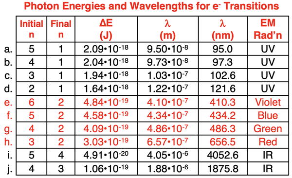
The table below includes calculations of the energy changes for a variety of electron transitions from an initial excited state to a lower energy state. The values used in the calculations were based on Bohr’s equation (E_n = -R_H / n²). These are Bohr’s predictions based on his quantum model of the atom. In the data table, Planck’s equation (E_photon = h•c / λ) was used to calculate the values of the photon’s wavelength (λ). The last column of the table shows the type of electromagnetic radiation that describes the photon. Rows e-h of the table are highlighted in red. These rows correspond to wavelengths in the visible light region of the spectrum. The other electron transitions result in photons that are not visible to the eye. Special instrumentation would be required to detect these photons.
 

 
As is the case with any new model (or old model), it must be asked how did Bohr do? That is, how well does the model fit the data? Is there good agreement between model and data? The data – the emission spectrum of hydrogen with the wavelength values for its four visible lines - is shown below.

 
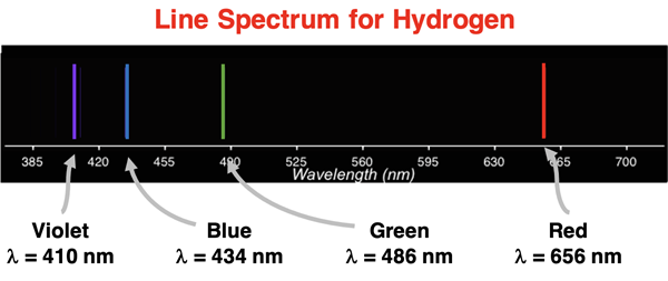
A comparison of rows e through h of the table to the values in the graphic demonstrated exceptional agreement between model and data.
 
 
 

 

Getting Closer

Bohr’s model fit the data for the hydrogen line spectra within approximately 0.1%. However, the model’s ability to fit the data for other elements was far worse than acceptable. Small adjustments to the model did not result in improvements. The general consensus was that the model was a step in the right direction. Quantized energy levels made sense for fitting spectra line data that had quantized emission lines. Further progress towards the modern model would have to wait for a bold hypothesis made by Louis de Broglie.
 
 
 

Before You Leave

• Refine your understanding of the Bohr model and try our Line Spectra Concept Builder.
• The Check Your Understanding section below include questions with answers and explanations. It provides a great chance to self-assess your understanding.

 
 
 

Check Your Understanding

Use the following questions to assess your understanding. Tap the Check Answer buttons when ready.
 

1. Let’s just suppose that on some other planet where energy units are quite different than our own,  that the energy of an electron in the n = 1 orbit is -180 units. What would be the energy of an electron in the n = 2 orbit? And in the n = 3 orbit?
(HINT: You will need to use the equation E = k/n², where k is the Rydberg constant equivalent for that planet.)

 
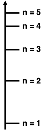
2. Consider the graphic at the right for the energy levels in the H atom. Assuming they are accurately scaled, how does the energy change compare for an electron transitioning between the two sets of initial and final states? Which of the transitions in each pair has the greatest ∆E?

1. n=5 to n=4  versus  n=5 to n=3
2. n=5 to n=4  versus  n=4 to n=3
3. n=5 to n=3  versus  n=3 to n=1

 

 
3. Consider the graphic at the right for the energy levels in the H atom. Assuming they are accurately scaled, how does the photon frequency compare for an electron transitioning between the two sets of initial and final states? Which of the transitions in each pair has the greatest photon frequency?

1. n=5 to n=4  versus  n=5 to n=3
2. n=5 to n=4  versus  n=4 to n=3
3. n=5 to n=3  versus  n=3 to n=1

 

 
4. Consider the graphic at the right for the energy levels in the H atom. Assuming they are accurately scaled, how does the photon wavelength compare for an electron transitioning between the two sets of initial and final states? Which of the transitions in each pair has the greatest photon wavelength?

1. n=5 to n=4  versus  n=5 to n=3
2. n=5 to n=4  versus  n=4 to n=3
3. n=5 to n=3  versus  n=3 to n=1

 


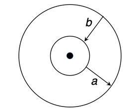
5. Bohr pictured electrons as orbiting the nucleus in circular orbits. Each orbit had its own energy level. Inner orbits have lower energy levels. Outer orbits have high energy levels. Atoms must __________ energy in order for electrons to move from inner to outer orbits (path a). And atoms must _________ energy for electrons to move from outer to inner orbits (path b).

1. create, destroy
2. destroy, create
3. absorb, release
4. release, absorb

 

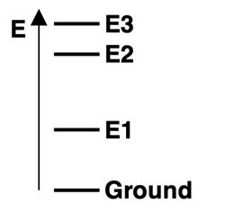
6. Consider the energy level diagram for atoms of Element X, showing the ground state and excited energy levels E1, E2, and E3. Three visible emission lines are observed for this element - red, blue, and violet. Based on the relative energy levels shown in the diagram, match these three colors to the corresponding transitions.
a. E1 State to Ground State:
Red      Blue    Violet
 
b. E2 State to Ground State:
Red      Blue    Violet
 
c. E3 State to E2 State:
Red      Blue    Violet