The Physics Classroom » Calculator Pad » Light Waves » Equation Overview

Waves, Sound and Light: Light Waves

Problem Sets || Overview of Physics || Legacy Problem Set

Light Waves: Problem Set Overview

There are 10 ready-to-use problem sets on the topic of Light Waves. The problems target your ability to determine wave quantities such as frequency, wavelength, and speed from verbal descriptions and diagrams of physical situations pertaining to wave propagation and wave interference. Problems range in difficulty from the very easy and straight-forward to the very difficult and complex.

The Speed of Light

The speed of any wave (v) is defined as the distance traveled (d) per time of travel (t) and is described by the following equation:

v = d / t

Thus, the distance traveled by a wave is related to the time required for it to travel that distance.

The speed of light, like the speed of any wave, is dependent upon the properties of the medium through which it is moving. For the problems in this problem set, the light waves are always moving through air or a vacuum. Unless told otherwise, a value of 2.998x10⁸ m/s should be used for the speed of light.

Frequency-Wavelength-Speed Relationship

Several questions in these problems target your ability to analyze physical situations involving the wavelength-frequency-speed relationship. Any wave, whether a smechanical wave or a light wave, will have a wavelength-frequency-speed relationship which follows the equation:

v = f • λ

where v represents the speed (or velocity) of the wave, f represents the frequency of the wave, and λ represents the wavelength of the wave. As mentioned above, a value of 2.998x10⁸ m/s should be used for the speed of light unless told otherwise.

The Doppler Effect

As a source of light waves (e.g., a star) moves toward or away from an observer, the frequency of the observed light is different than the actual source frequency. This phenomenon is known as the Doppler effect. As the source of the light waves approaches you, there is an upward shift in the observed frequency relative to the source frequency. And as the source of light waves moves away from you, there is a downward shift in the observed frequency relative to the source frequency. The frequency (f') that is observed can be calculated by using the Doppler Shift equations.

f' = f / (1 ± v_s/v)

where v = the speed of light, v_s = the speed at which the light source move, f = the frequency of the source, and f' = observed frequency. In the denominator of this equation, the minus sign is used for situations in which the source is approaching the observer and the plus sign is used in situations in which the source is moving away from the observer.

The same phenomenon would be observed when the observer is approaching a stationary source or moving away from the stationary source. Once more, the frequency that is heard can be calculated by using the Doppler Shift equations.

f' = (1 ± vo/v)•f

where v = the speed of light, v_o = the speed of the observer, f = the frequency of the source, and f' = observed frequency. In this equation, the plus sign is used for situations in which the observer is approaching the source and the minus sign is used in situations in which the observer is moving away from the source.

Radar guns present a more difficult challenge. Let's consider the case of the radar gun being stationary (in a police car) along the side of the road. The radar (light waves) are emitted by the gun, travel towards an oncoming or departing vehicle, bounce off the vehicle, and return to the radar gun for detection. So the original source of light waves is the radar gun and the final observer of light waves is the radar gun. The radar gun is stationary at all times. But in between the sending and receiving of the light waves, the waves reflect off a moving vehicle. The frequency of the reflected waves is equal to the observed frequency that the vehicle would observe. In the end, there are two Doppler shifts - the one that occurs for the moving vehicle (because it is moving towards or away from the stationary light source) and the one that occurs for the stationary radar gun (because it perceives waves that are reflected by the vehicle that is either moving towards or away from it). So the solution to the radar gun.

Two Point Source Interference Patterns

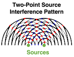The diagram at the right depicts an interference pattern produced by two periodic waves (water waves, sound waves, light waves, etc.). The crests are denoted by the thick lines and the troughs are denoted by the thin lines. Constructive interference occurs wherever a thick line meets a thick line or a thin line meets a thin line; this type of interference results in the formation of an antinode. The antinodes are denoted by red dots. Destructive interference occurs wherever a thick line meets a thin line; this type of interference results in the formation of a node. The nodes are denoted by blue dots. The pattern is a standing wave pattern, characterized by the presence of nodes and antinodes which are standing still - i.e., always located at the same position on the medium. The antinodes (points where the waves interfere constructively) seem to be located along lines - creatively called antinodal lines. The nodes also fall along lines - called nodal lines. The two-point source interference pattern is characterized by a pattern of alternating nodal and antinodal lines. The central line in the pattern - the line which bisects the line segment which is drawn between the two sources is an antinodal line. This central antinodal line is a point where the waves from each source reinforce each other by means of constructive interference.

The nodal and antinodal points in the interference pattern result when light from two different sources travel two different distances to the same point in the pattern in such a manner that destructive or constructive interference occurs at that point. The fact that the two waves travel two different distances means that there is a path difference - a difference in distance traveled by the two waves from the source. If the path difference is equal to some whole number of wavelengths, then a crest from one source will meet a crest from the other source (or a trough will meet a trough) and constructive interference will occur at that point. If the path difference is a half-number of wavelengths, then a crest from one source will meet a trough from the other source and destructive interference will occur at that point. This truth can be expressed mathematically by the following equation

PD = m • λ
m = 0, 1, 2, 3, ... for antinodal lines
m = 0.5, 1.5, 2.5, 3.5 ... for nodal lines

where PD is the path difference, λ is the wavelength, and m is the so-called order number of the line that the particular point lies along. Since the path difference is the difference in distance traveled from a source to the point on the line (nodal or antinodal), the equation above is sometimes written as

PD = | S₁P - S₂P | = m • λ

where S₁P is the distance from source 1 to the point P and S₂P is the distance from source 2 to point P. This equation will be used several times in these problems.

Young's Equation

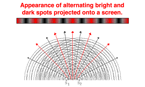
The diagram above depicts the two-dimensional pattern of water waves, sound waves or light waves spreading out over two-dimensional space to create a pattern of nodal and antinodal lines. If the sources creating the pattern are monochromatic and coherent light sources, then each nodal line would be representative of a collection of dark spots (destructive interference) and each antinodal line would be representative of a collection of bright spots (constructive interference). If this pattern were projected onto a screen at a given distance L from the sources, then there would be an appearance of alternating dark and bright spots on the screen. This is depicted in the diagram below.

In the early 19th century, physicist Thomas Young noted that there would be some observable and measurable distances evident in the pattern which would be mathematically related to the wavelength of the laser light. Young's famous equation, shown below, related these measurable quantities to the wavelength of light (λ).

λ = y•d / (m•L)

where d is the separation distance between the sources, L is the distance from the sources to the screen, m is the order number of the nodal or antinodal line and y is the distance between the central antinodal line and a point on the mth-order nodal or antinodal line. The m in the above equation is the same m used in the path difference equation. It will be a whole number for antinodal lines and a half-number for nodal line. Once a point on a nodal or antinodal line is selected, m is determined and the measurement of y, d and L can be made. Once made, the wavelength of the light waves can be calculated. The above equation is used frequently throughout these problems.

A more detailed and exhaustive discussion of two point source interference patterns and Young's Equation can be found at The Physics Classroom Tutorial.

Being Successful at Solving Two Point Source Interference Problems

Success at solving two point source interference problems demands an understanding of the above concepts and mathematics. But it also demands that you develop and practice the following skills:

read a physical description of a two-point source interference situation and appropriately extract numerical information from it.
give attention to units and have a plan for converting units in such a manner that the unknown quantity is expressed in the requested units. You should know that: 10² cm = 1 m; 10³ mm = 1 m; 10⁹ nm = 1 m; and 10¹⁰ Angstroms = 1 m.
know the meaning of the variables (λ, y, d, m, L, PD) in the equations discussed above.
understand that the spacing between bright and dark spots on the screen is regular and repeating such that the distance between the central antinodal position and the third antinodal position is roughly three times the distance between the central antinodal position and the first antinodal position.
understand the order numbering system used to describe a projected pattern.
practice the habits of an effective problem-solver.

Habits of an Effective Problem-Solver

An effective problem solver by habit approaches a physics problem in a manner that reflects a collection of disciplined habits. While not every effective problem solver employs the same approach, they all have habits which they share in common. These habits are described briefly here. An effective problem-solver...

...reads the problem carefully and develops a mental picture of the physical situation. If needed, they sketch a simple diagram of the physical situation to help visualize it.
...identifies the known and unknown quantities and records them in an organized manner, often times recording them on the diagram itself. They equate given values to the symbols used to represent the corresponding quantity (e.g., v = 3.00x10⁸ m/s, λ = 554 nm, f = ???).
...plots a strategy for solving for the unknown quantity; the strategy will typically center around the use of physics equations and be heavily dependent upon an understanding of physics principles.
...identifies the appropriate formula(s) to use, often times writing them down. Where needed, they perform the needed conversion of quantities into the proper unit.
...performs substitutions and algebraic manipulations in order to solve for the unknown quantity.

Additional Readings/Study Aids:

The following pages from The Physics Classroom Tutorial may serve to be useful in assisting you in the understanding of the concepts and mathematics associated with these problems.